1. Introduction

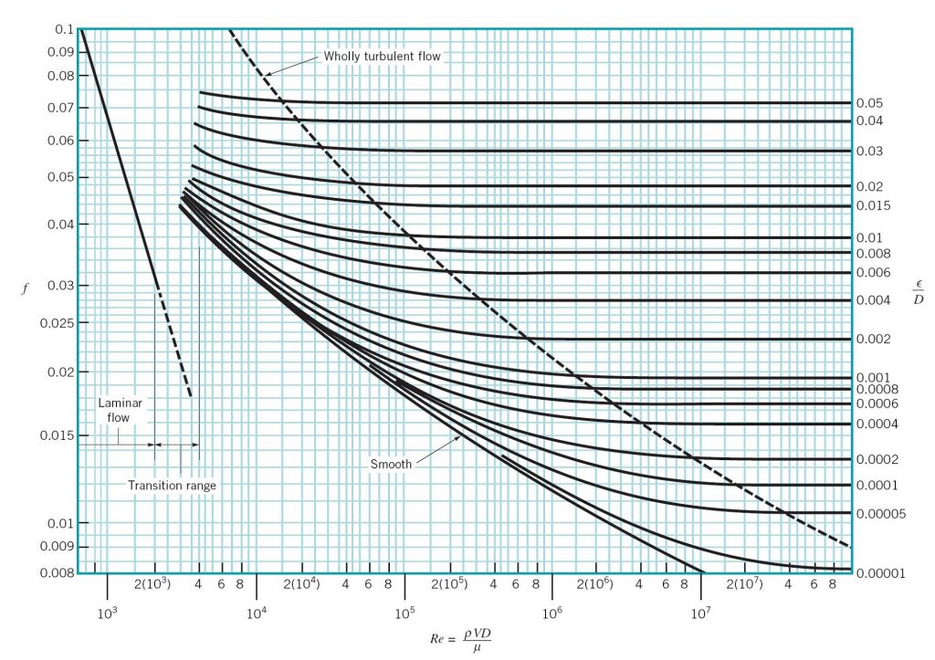
The total energy loss in a pipe system is the sum of the major and minor losses. Major losses are associated with frictional energy loss that is caused by the viscous effects of the fluid and roughness of the pipe wall. Major losses create a pressure drop along the pipe since the pressure must work to overcome the frictional resistance. The Darcy-Weisbach equation is the most widely accepted formula for determining the energy loss in pipe flow. In this equation, the friction factor (f ), a dimensionless quantity, is used to describe the friction loss in a pipe. In laminar flows, f is only a function of the Reynolds number and is independent of the surface roughness of the pipe. In fully turbulent flows, f depends on both the Reynolds number and relative roughness of the pipe wall. In engineering problems, f is determined by using the Moody diagram.

2. Practical Application

In engineering applications, it is important to increase pipe productivity, i.e. maximizing the flow rate capacity and minimizing head loss per unit length. According to the Darcy-Weisbach equation, for a given flow rate, the head loss decreases with the inverse fifth power of the pipe diameter. Doubling the diameter of a pipe results in the head loss decreasing by a factor of 32 (≈ 97% reduction), while the amount of material required per unit length of the pipe and its installation cost nearly doubles. This means that energy consumption, to overcome the frictional resistance in a pipe conveying a certain flow rate, can be significantly reduced at a relatively small capital cost.

3. Objective

The objective of this experiment is to investigate head loss due to friction in a pipe, and to determine the associated friction factor under a range of flow rates and flow regimes, i.e., laminar, transitional, and turbulent.

4. Method

The friction factor is determined by measuring the pressure head difference between two fixed points in a straight pipe with a circular cross section for steady flows.

5. Equipment

The following equipment is required to perform the energy loss in pipes experiment:

F1-10 hydraulics bench,
F1-18 pipe friction apparatus,
Stopwatch for timing the flow measurement,
Measuring cylinder for measuring very low flow rates,
Spirit level, and
Thermometer.

6. Equipment Description

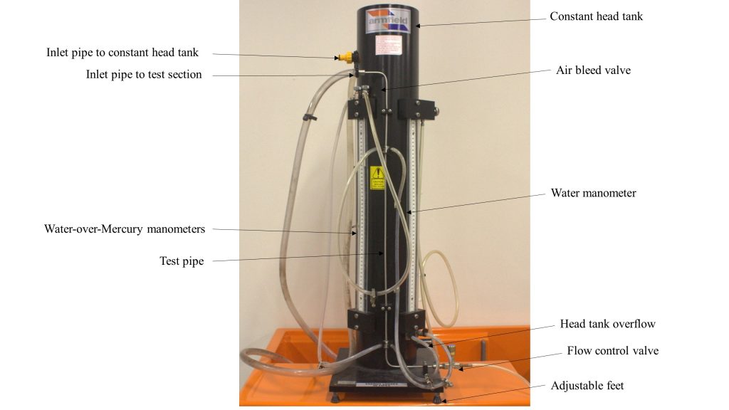
The pipe friction apparatus consists of a test pipe (mounted vertically on the rig), a constant head tank, a flow control valve, an air-bleed valve, and two sets of manometers to measure the head losses in the pipe (Figure 4.1). A set of two water-over-mercury manometers is used to measure large pressure differentials, and two water manometers are used to measure small pressure differentials. When not in use, the manometers may be isolated, using Hoffman clamps.

Since mercury is considered a hazardous substance, it cannot be used in undergraduate fluid mechanics labs. Therefore, for this experiment, the water-over-mercury manometers are replaced with a differential pressure gauge to directly measure large pressure differentials.

This experiment is performed under two flow conditions: high flow rates and low flow rates. For high flow rate experiments, the inlet pipe is connected directly to the bench water supply. For low flow rate experiments, the inlet to the constant head tank is connected to the bench supply, and the outlet at the base of the head tank is connected to the top of the test pipe [4].

The apparatus’ flow control valve is used to regulate flow through the test pipe. This valve should face the volumetric tank, and a short length of flexible tube should be attached to it, to prevent splashing.

The air-bleed valve facilitates purging the system and adjusting the water level in the water manometers to a convenient level, by allowing air to enter them.

Diagram for F1-18 Pipe Friction Test Apparatus. The constant head tank sits at the top of the apparatus. On the left hand side of the apparatus beneath the constant head tank is the inlet pipe to constant head tank and the inlet pipe to test section. Beneath the inlet pipe to test section is the <a href= air bleed valve. The water manometer connects to the air bleed valve and runs down to the base of the apparatus. On the bottom left hand side of the apparatus sits the water-over-mercury manometers and the test pipe, and on the bottom right hand rests the head tank overflow and the flow control valve." width="856" height="482" />

7. Theory

The energy loss in a pipe can be determined by applying the energy equation to a section of a straight pipe with a uniform cross section:

$\frac{P_{in}}{\gamma}+\frac{v_{in}^2}{2g}+z_{in}=\frac{P_{out}}{\gamma}+\frac{v_{out}^2}{2g}+z_{out}+h_L\qquad (1)$

If the pipe is horizontal:

$h_L=\frac{(P_{out}-P_{in})}{\gamma}\qquad (2)$

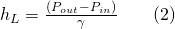
The pressure difference (P_out-P_in) between two points in the pipe is due to the frictional resistance, and the head loss h_L is directly proportional to the pressure difference.

The head loss due to friction can be calculated from the Darcy-Weisbach equation:

: head loss due to flow resistance

f: Darcy-Weisbach coefficient

D: pipe diameter

v: average velocity

g: gravitational acceleration.

For laminar flow, the Darcy-Weisbach coefficient (or friction factor f ) is only a function of the Reynolds number (Re) and is independent of the surface roughness of the pipe, i.e.:

$f=\frac{64}{Re}\hphantom{abcdefghij}(Hagen-Poiseuille\,equation)\qquad (4)$

For turbulent flow, f is a function of both the Reynolds number and the pipe roughness height, . Other factors, such as roughness spacing and shape, may also affect the value of f; however, these effects are not well understood and may be negligible in many cases. Therefore, f must be determined experimentally. The Moody diagram relates f to the pipe wall relative roughness ( /D) and the Reynolds number (Figure 4.2).

Instead of using the Moody diagram, f can be determined by utilizing empirical formulas. These formulas are used in engineering applications when computer programs or spreadsheet calculation methods are employed. For turbulent flow in a smooth pipe, a well-known curve fit to the Moody diagram is given by:

$f=0.316Re^{-0.25} \hphantom{abcdefghij}(Blasius\enspace equation)\qquad (5)$

Reynolds number is given by:

$Re=\frac{\rho vD}{\mu}=\frac{vD}{\nu}\qquad (6)$

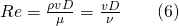
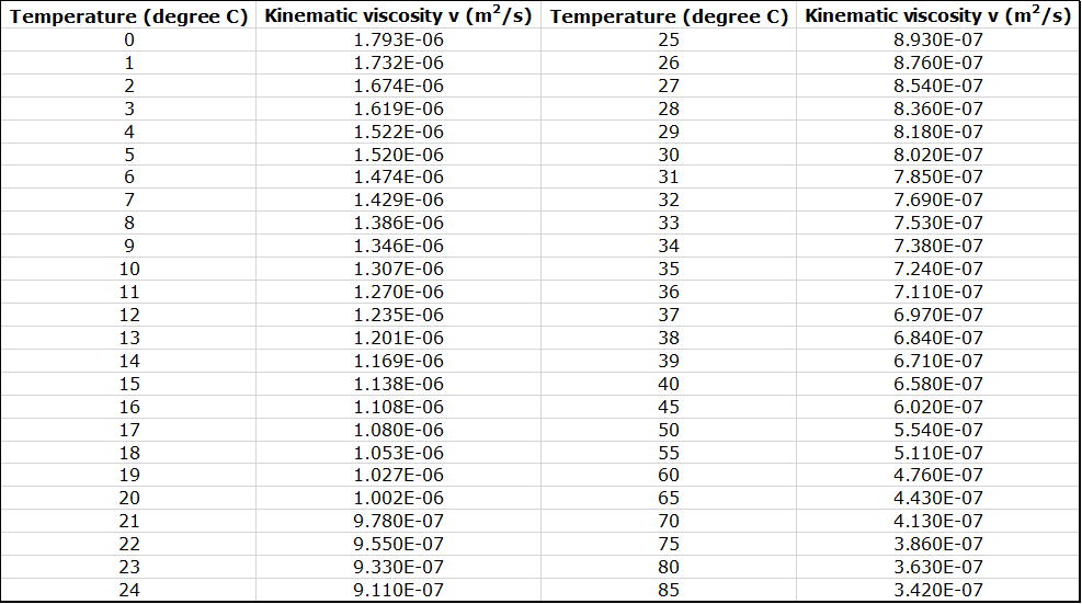
where v is the average velocity, D is the pipe diameter, and and are dynamic and kinematic viscosities of the fluid, respectively. (Figure 4.3).

In this experiment, h_L is measured directly by the water manometers and the differential pressure gauge that are connected by pressure tappings to the test pipe. The average velocity, v, is calculated from the volumetric flow rate (Q ) as:

The following dimensions from the test pipe may be used in the appropriate calculations [4]:

Length of test pipe = 0.50 m,

Diameter of test pipe = 0.003 m.

An example of a Moody Diagram Table of Kinematic Viscosity of Water (v) at Atmospheric Pressure. The first column displays temperature in degrees celsius from 0 to 25. The second column displays kinematic viscosity (v) in meters squared per sec. The third column displays temperature in degrees celsius from 25 to 85. The fourth column displays kinematic viscosity (v) in meters squared per sec.

8. Experimental Procedure

The experiment will be performed in two parts: high flow rates and low flow rates. Set up the equipment as follows:

Mount the test rig on the hydraulics bench, and adjust the feet with a spirit level to ensure that the baseplate is horizontal and the manometers are vertical.
Attach Hoffman clamps to the water manometers and pressure gauge connecting tubes, and close them off.

High Flow Rate Experiment

The high flow rate will be supplied to the test section by connecting the equipment inlet pipe to the hydraulics bench, with the pump turned off. The following steps should be followed.

Close the bench valve, open the apparatus flow control valve fully, and start the pump. Open the bench valve progressively, and run the flow until all air is purged.
Remove the clamps from the differential pressure gauge connection tubes, and purge any air from the air-bleed valve located on the side of the pressure gauge.
Close off the air-bleed valve once no air bubbles observed in the connection tubes.
Close the apparatus flow control valve and take a zero-flow reading from the pressure gauge.
With the flow control valve fully open, measure the head loss shown by the pressure gauge.
Determine the flow rate by timed collection.
Adjust the flow control valve in a step-wise fashion to observe the pressure differences at 0.05 bar increments. Obtain data for ten flow rates. For each step, determine the flow rate by timed collection.
Close the flow control valve, and turn off the pump.

The pressure difference measured by the differential pressure gauge can be converted to an equivalent head loss (h_L) by using the conversion ratio:

1 bar = 10.2 m water

Low Flow Rate Experiment

The low flow rate will be supplied to the test section by connecting the hydraulics bench outlet pipe to the head tank with the pump turned off. Take the following steps.

Attach a clamp to each of the differential pressure gauge connectors and close them off.
Disconnect the test pipe’s supply tube and hold it high to keep it filled with water.
Connect the bench supply tube to the head tank inflow, run the pump, and open the bench valve to allow flow. When outflow occurs from the head tank snap connector, attach the test section supply tube to it, ensuring that no air is entrapped.
When outflow occurs from the head tank overflow, fully open the control valve.
Remove the clamps from the water manometers’ tubes and close the control valve.
Connect a length of small bore tubing from the air valve to the volumetric tank, open the air bleed screw, and allow flow through the manometers to purge all of the air from them. Then tighten the air bleed screw.
Fully open the control valve and slowly open the air bleed valve, allowing air to enter until the manometer levels reach a convenient height (in the middle of the manometers), then close the air vent. If required, further control of the levels can be achieved by using a hand pump to raise the manometer air pressure.
With the flow control valve fully open, measure the head loss shown by the manometers.
Determine the flow rate by timed collection.
Obtain data for at least eight flow rates, the lowest to give h_L= 30 mm.
Measure the water temperature, using a thermometer.

9. Results and Calculations

Please use this link for accessing excel workbook for this experiment.

9.1. Results

Record all of the manometer and pressure gauge readings, water temperature, and volumetric measurements, in the Raw Data Tables.

Raw Data Tables: High Flow Rate Experiment

Test No.	Head Loss (bar)	Volume (Liters)	Time (s)
1
2
3
4
5
6
7
8
9
10

Raw Data Tables: Low Flow Rate Experiment

Test No.	h₁ (m)	h₂ (m)	Head loss h_L (m)	Volume (liters)	Time (s)
1
2
3
4
5
6
7
8
Water Temperature:

9.2. Calculations

Calculate the values of the discharge; average flow velocity; and experimental friction factor, f using Equation 3, and the Reynolds number for each experiment. Also, calculate the theoretical friction factor, f, using Equation 4 for laminar flow and Equation 5 for turbulent flow for a range of Reynolds numbers. Record your calculations in the following sample Result Tables.

Result Table- Experimental Values

Test No.	Head loss h_L (m)	Volume (liters)	Time (s)	Discharge (m 3 /s)	Velocity (m/s)	Friction Factor, f	Reynolds Number
1
2
3
4
5
6
7
8
9
10
11
12
13
14
15
16
17
18

Result Table- Theoretical Values

No.	Flow Regime	Reynolds Number	Friction Factor, f
1	Laminar (Equation 4)	100
2		200
3		400
4		800
5		1600
6		2000
7	Turbulent (Equation 5)	4000
8		6000
9		8000
10		10000
11		12000
12		16000
13		20000

10. Report

Use the template provided to prepare your lab report for this experiment. Your report should include the following:

Table(s) of raw data
Table(s) of results
Graph(s)
- On one graph, plot the experimental and theoretical values of the friction factor, f (y-axis) against the Reynolds number, Re (x-axis) on a log-log scale. The experimental results should be divided into three groups (laminar, transitional, and turbulent) and plotted separately. The theoretical values should be divided into two groups (laminar and turbulent) and also plotted separately.
- On one graph, plot h_L (y-axis) vs. average flow velocity, v (x-axis) on a log-log scale.

Discuss the following:
- Identify laminar and turbulent flow regimes in your experiment. What is the critical Reynolds number in this experiment (i.e., the transitional Reynolds number from laminar flow to turbulent flow)?
- Assuming a relationship of the form , calculate K and n values from the graph of experimental data you have plotted, and compare them with the accepted values shown in the Theory section (Equations 4 and 5). What is the cumulative effect of the experimental errors on the values of K and n?
- What is the dependence of head loss upon velocity (or flow rate) in the laminar and turbulent regions of flow?
- What is the significance of changes in temperature to the head loss?
- Compare your results for f with the Moody diagram (Figure 4.2). Note that the pipe utilized in this experiment is a smooth pipe. Indicate any reason for lack of agreement.
- What natural processes would affect pipe roughness?